Disclaimer
All materials and contents are provided for information purposes only. Moscow Exchange assumes no obligations, and makes no representations or warranties, whether express or implied, with regard to the accuracy, completeness, quality, merchantability, correctness, compliance with any specific methodologies and descriptions or the fitness for any particular purpose as well as volume, structure, format, submission dates and timeliness, of such materials and contents. Any such materials and contents (or any portion thereof) cannot be used for any investment or commercial purposes including the creation of financial instruments, products or indices.
Aggregated Netflow Analytics 1
Description
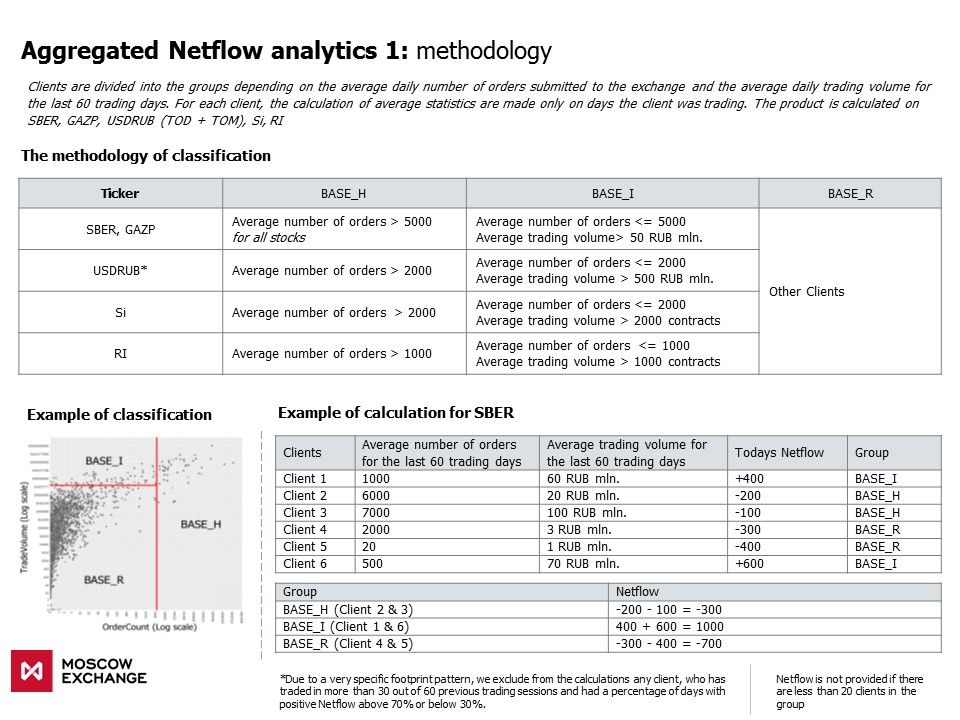
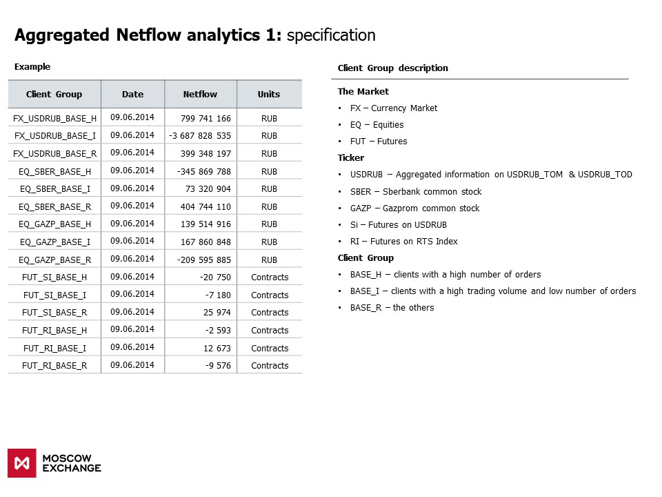
The product contains netflow(difference between buy and sell volume) for each of the following groups:
- BASE_H - clients with a high number of orders
- BASE_I - clients with a high trading volume and a low number of orders
- BASE_R - the others
Netflow is calculated for the following instruments:
- SBER
- GAZP
- USDRUB
- Si
- RI
#libs import
import pandas as pd
import matplotlib.pyplot as plt
import seaborn as sns
import numpy as np
from scipy.stats import spearmanr

%matplotlib inline
sns.set_style("dark")
plt.rcParams['figure.figsize'] = (15, 7)

# colors
graphcolors = {'red'    :'#c8102e',
               'grey'   :'#51626f',
               'blue'   :'#0070c0',
               'orange' :'#ffa100',
               'green'  :'#00b050',
               'black'  :'#000000',
               'white'  :'#ffffff'}
Data Review
df = pd.read_csv('all_instruments.csv', parse_dates = ['SESSIONID'], index_col = 'SESSIONID')
df.head()
df.tail()
The columns names include:
- FUT, EQ, FX - market
- RI, SBER, USDRUB, GAZP, Si - instrument
- BASE_H, BASE_I, BASE_R - client group
Hypothesis testing. Is netflow correlated with price?
SBER
cl_groups = ['BASE_H', 'BASE_I', 'BASE_R']
sber_df = pd.DataFrame(index = df.index)
for gr in cl_groups:
    sber_df[gr] = df['EQ_SBER_' + gr]
sber_df.head()
# reading the prices
sber_ohlc = pd.read_csv('Price_SBER.csv', index_col= 0, parse_dates = ['begin', 'end'])
sber_ohlc.head(2)
#close auction prices
close_auction = sber_ohlc[(sber_ohlc['begin'].dt.hour == 18) & (sber_ohlc['begin'].dt.minute == 30)].copy()
close_auction.begin = close_auction.begin.map(lambda x: x + pd.Timedelta(hours = -x.hour, minutes = -x.minute, seconds = -x.second))
close_auction = close_auction.set_index('begin')[['close']]
close_auction.index.name = 'SESSIONID'
close_auction.head()
sber_df['close_auction_price'] = close_auction.close
sber_df.head()
sber_df[['BASE_H', 'BASE_I', 'BASE_R']].cumsum().plot()
sber_df.close_auction_price.plot(secondary_y= True, label = 'price', color = 'orange')
plt.legend(loc = (0.005, 0.81))
plt.show()

We can see that there is correlation between SBER price and BASE_H
sber_df['price_chng'] = sber_df.close_auction_price.pct_change()
sber_df.corr()
Let's examine correlation between Netflows and close-to-close next day return. For each of the BASE_H, BASE_I, BASE_R we will set up a hypothesis H0, stating that there is no correlation between next day return and Netflow. The alternative hypothesis H1 states that the correlation is not zero. We will test this hypothesis using 5% significance level.
sber_df['next_price_chng'] = sber_df.price_chng.shift(-1)
sber_df = sber_df.dropna()
for g in ['BASE_H', 'BASE_I', 'BASE_R']:
    scor = spearmanr(sber_df[g], sber_df['next_price_chng'])
    if np.abs(scor[1]) < 0.05:
        print('H0 is rejected, correlation between {0} and next day return is'.format(g),
              round(scor[0], 3),'; p-value:', round(scor[1], 3))
    else:
        print('H0 is not rejected, correlation between {0} and next day return is'.format(g),
              round(scor[0], 3),'; p-value:', round(scor[1], 3))
We can reject the hypothesis H0 about zero correlation between BASE_H and SBER next day return as well as BASE_R and SBER next day return at the 5% significance level.
USDRUB
cols = [x for x in df.columns if x[:6] == 'FUT_SI' or x[:2] == 'FX']
usdrub_df = df[cols].copy()

usdrub_ohlc = pd.read_csv('Price_USDRUB.csv', index_col= 0, parse_dates = ['begin', 'end'])
close_auction = usdrub_ohlc[(usdrub_ohlc['begin'].dt.hour == 18) & (usdrub_ohlc['begin'].dt.minute == 30)].copy()
close_auction.begin = close_auction.begin.map(lambda x: x + pd.Timedelta(hours = -x.hour, minutes = -x.minute, seconds = -x.second))
close_auction = close_auction.set_index('begin')[['close']]
close_auction.index.name = 'SESSIONID'
usdrub_df['close_auction_price'] = close_auction.close
fx_cols = [x for x in df.columns if x[:2] == 'FX']
usdrub_df[fx_cols].cumsum().plot()
usdrub_df.close_auction_price.plot(secondary_y= True, label = 'price', color = 'orange')
plt.legend(loc = (0.005, 0.81))
plt.show()

fut_cols = [x for x in df.columns if x[:6] == 'FUT_SI']
usdrub_df[fut_cols].cumsum().plot()
usdrub_df.close_auction_price.plot(secondary_y= True, label = 'price', color = 'orange')
plt.legend(loc = (0.005, 0.81))
plt.show()

usdrub_df['price_chng'] = usdrub_df.close_auction_price.pct_change()
usdrub_df.corr()
Return is correlated with FX_USDRUB_BASE_R, FUT_SI_BASE_H, FUT_SI_BASE_R
usdrub_df['next_price_chng'] = usdrub_df.price_chng.shift(-1)
usdrub_df = usdrub_df.dropna()
for g in cols:
    scor = spearmanr(usdrub_df[g], usdrub_df['next_price_chng'])
    if np.abs(scor[1]) < 0.05:
        print('H0 is rejected, correlation between {0} and next day return is'.format(g),
              round(scor[0], 3),'; p-value:', round(scor[1], 3))
    else:
        print('H0 is not rejected, correlation between {0} and next day return is'.format(g),
              round(scor[0], 3),'; p-value:', round(scor[1], 3))
We can reject the hypothesis H0 about zero correlation between FX_USDRUB_BASE_H, FUT_SI_BASE_H, FUT_SI_BASE_I , FUT_SI_BASE_R and the USDRUB next day return at the 5% significance level.
Contacts
Website - https://moex.com/en/analyticalproducts?netflow1
Email - support.dataproducts@moex.com