Disclaimer
All materials and contents are provided for information purposes only. Moscow Exchange assumes no obligations, and makes no representations or warranties, whether express or implied, with regard to the accuracy, completeness, quality, merchantability, correctness, compliance with any specific methodologies and descriptions or the fitness for any particular purpose as well as volume, structure, format, submission dates and timeliness, of such materials and contents. Any such materials and contents (or any portion thereof) cannot be used for any investment or commercial purposes including the creation of financial instruments, products or indices.
Content:
- Brief product description
- Methodology
- Fields description
- Data review
- Creating derived features
- Direction of netflow and tomorrow price movement
- Resume
- Contacts
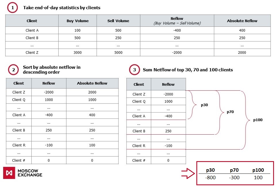
Brief product description
The product includes aggregated daily netflow (buy volume - sell volume) of top 30, 70 and 100 clients by absolute value of netflow in number of shares and RUB. All trades of all clients in order driven trading mode starting from 10:00 A.M. till to 6:30 P.M. are taken into account for calculations. At 6:30 P.M. the clients with a highest absolute value of netflow are selected and their netflows are summarized. At the end of the day there are three values for top 30, 70 and 100 clients in number of shares and in RUB.
Currently netflow values available for the following 10 equities: SBER, GAZP, LKOH, GMKN, VTBR, ROSN, MGNT, ALRS, SBERP, AFLT
Methodology
Fields description
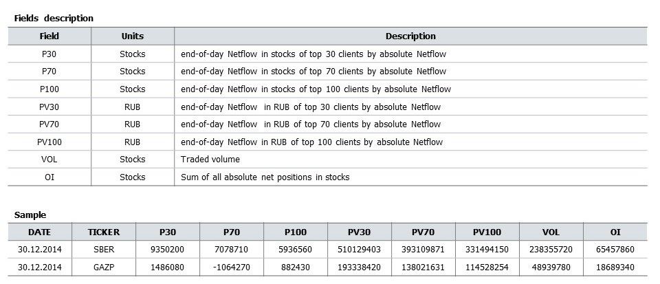
Key defenitions used below:
- p30, p70, p100 - Aggregated netflow by 30, 70 and 100 clients, in shares
- today_change - today's price change (today's close to open), in %
- tomorrow_change - tomorrow's price change (tomorrow's close to today's close), in %
Data review
import pandas as pd
import numpy as np
import matplotlib.pyplot as plt
%pylab inline
plt.rcParams['figure.figsize'] = (15, 8)
plt.style.use('ggplot')
Let's consider data on SBER equity (Sberbank of Russia). We will read historical values of netflow for 4 years (2014-2017)
ticker = 'SBER'
X = pd.read_csv('../netflows_2014_2017/' + ticker + '_netflow.csv')
X['date'] = pd.to_datetime(X['date'])
X = X.set_index('date')
X = X[['p30', 'p70', 'p100', 'oi']][3:]
X.head()
# Key statistics
X.describe()
# Time-Series chart. Cumulative amount of p30, p70 and p100
X[['p30', 'p70', 'p100']].cumsum().rolling(5).mean().plot()

# Distribution of values p30, p70 and p100. Average and median values ~0
X[['p30', 'p70', 'p100']].plot.box()

Let's calculate the correlations between p30, p70, p100 and today_change, tomorrow_change. Downloading historical prices and volumes - OHLCV:
# function to get OHLCV daily values for a given ticker and for a given time period using MOEX API
def get_ohlcv(ticker, date_from, date_till):
    P = pd.DataFrame()

    # using 'for' loop because max outputs are limited by 500 rows
    for i in range(5):
        url = 'http://iss.moex.com/iss/engines/stock/markets/shares/boards/tqbr/securities/' + ticker + '/candles.csv' \
        '?from=' + date_from + \
        '&till=' + date_till + \
        '&interval=24' \
        '&start=' + str(500*i)
        P = P.append(pd.read_csv(url, ';',skiprows=2))
    P['date'] = P.apply(lambda row: row['begin'][:10], axis =1)
    P['date'] = pd.to_datetime(P['date'], format = '%Y-%m-%d')
    P = P.set_index('date')

    #subtracting by 2, to get Turnover from Volume
    P['volume'] = 2 * P['volume']
    P['value'] = 2 * P['value']

    P.drop(['begin', 'end'], axis = 1, inplace = True)
    return P
Y = get_ohlcv(ticker, '2014-01-01', '2018-01-30')
# change - today's price change (close to open)
Y['today_change'] = 100 * (Y['close'] - Y['open']) / Y['open']

# tom_change - tomorrow's price change (close(+1) to сlose(0))
Y['tomorrow_change'] = 100 * Y['close'].pct_change().shift(-1)

Y.head()
# Adding price changes to the netflow data frame
X = pd.merge(X, Y[['today_change', 'tomorrow_change', 'volume', 'value']], how='left', left_index = True, right_index = True)
X.head()
# Time-Series chart. Cumulative amount of p30, p70, p100 and today's price change - today_change (black line)
X[['p30', 'p70', 'p100']].cumsum().rolling(5).mean().plot()
plt.ylabel('Number of shares')
X['today_change'].cumsum().rolling(5).mean().plot(secondary_y = True, c='#000000')
plt.ylabel('%')

Correlation between p30, p70, p100 and today_change, tommorow_change for 4 years
X[['p30', 'p70', 'p100', 'today_change', 'tomorrow_change']].corr()
- Strong correlation between p30, p70 and p100 (~0.98)
- Strong positive correlation between p30, p70, p100 and today_change (~0.75)
- Weak positive correlation between p30, p70, p100 and tomorrow_change (~0.09)
Therefore, it can be assumed that today_change is connected with p30, p70 and p100. Also, there is weak stable connection between netflow and tommorow_change.
Maybe it is possible to increase correlation between p30, p70, p100 and tommorow_change:
- Let's normalize p30, p70 и p100 on trading volume - VOLUME (OI, log(VOLUME) ...)
- Calculate p30, p70 и p100 changes regarding previous N days.
Creating derived features
Z = X.copy()
Z['p30_vol'] = 100 * Z['p30'] / Z['volume']
Z['p70_vol'] = 100 * Z['p70'] / Z['volume']
Z['p100_vol'] = 100 * Z['p100'] / Z['volume']
Z = Z.astype(float)
Z.corr()
When p30, p70, p100 are normalized on volume, correlation between p30_vol, p70_vol, p100_vol and tomorrow_change became ~0.1
Let's calculate difference(delta) of p30, p70 and p100 regarding their average for previous 1-5 days
cols = ['p30', 'p70', 'p100', 'p30_vol', 'p70_vol', 'p100_vol']

for col in cols:
    for i in [1,2,3,4,5]:
        Z[col + '_' + str(i)] = Z[col] - Z[col].shift(periods=1, freq=None, axis=0).rolling(i, min_periods = 1).mean()

print('New table shape ' + str(Z.shape))
Z.head()
# top 10 most correlated features
cols = Z.corr()['tomorrow_change'].sort_values(ascending = False)[1:11]

cols
Differences of p30, p70 and p100 shows correlation of ~0.11. Correlations on other instruments are in the table below.
| TICKER | POS vs TOD_CHG | POS vs TOM_CHG | POS/VOL vs TOM_CHG | ΔPOS/VOL vs TOM_CHG |
|---|---|---|---|---|
| SBER | 0.75 | 0.09 | 0.10 | 0.11 |
| GAZP | 0.73 | 0.09 | 0.08 | 0.11 |
| LKOH | 0.65 | 0.08 | 0.08 | 0.13 |
| GMKN | 0.60 | 0.04 | 0.07 | 0.05 |
| MGNT | 0.60 | 0.04 | 0.07 | 0.06 |
| ROSN | 0.67 | 0.10 | 0.11 | 0.12 |
| VTBR | 0.56 | 0.10 | 0.01 | 0.06 |
| ALRS | 0.45 | 0.00 | 0.04 | 0.07 |
| SBERP | 0.50 | 0.07 | 0.10 | 0.09 |
| AFLT | 0.50 | 0.06 | 0.07 | 0.07 |
- POS vs TOD_CHG - correlation between netflow and today_change
- POS vs TOM_CHG - correlation between netflow and tomorrow_change
- POS/VOL vs TOM_CHG - correlation between netflow (divided on volume) and tomorrow_change
- ΔPOS/VOL vs TOM_CHG - correlation between netflow differences (deltas) over previous days and tomorrow_change
One can examine correlation over 4 years.
Сo-directionality of netflow and tommorow_change statistics
Averages of p30, p70 and p100 and their differencies are located near zero. Let's calculate co-directionality statistics of netflow and tommorow_change in days and percentages based on p70_vol_3 (correlation with tommorow-change ~ 0.11):
*difference between p70 normalized on volume and its average over the 3 previous days
Z = Z[1:]
Z = Z[Z['tomorrow_change'] != 0]
Z['feature'] = np.sign(Z['p70_vol_3'])
Z['base'] = np.sign(Z['tomorrow_change'])
pd.crosstab(index = Z['feature'].astype(int), columns = Z['base'].astype(int))
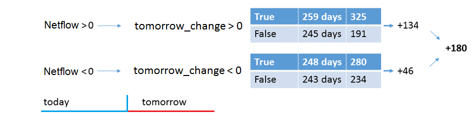
- 248 - Number of days when netflow and tommorow_change are negative (co-directional)
- 259 - Number of days when netflow and tommorow_change are positive (co-directional)
- 243 - Number of days when netflow is negative and tomorrow_change is positive (oppositely directed)
- 245 - Number of days when netflow is positive and tomorrow_change is negative (oppositely directed)
In the same way, let's calculate cumulative sum of price percentage changes in case of co-directionality and opposite directionality:
pd.crosstab(index = Z['feature'].astype(int), columns = Z['base'].astype(int), values = Z['tomorrow_change'].abs().astype(int), aggfunc = 'sum')
- 280 - Netflow and tomorrow_change are negative
- 325 - Netflow and tomorrow_change are positive
- 234 - Netflow is negative and tomorrow_change is positive
- 191 - Netflow is positive and tomorrow_change is negative
When netflow and tomorrow_change are co-directed, price change sum = 615 (280+325), when opposite directed = 425 (234+191)
Co-directionality statistics based on p70_vol_3 equals 180 (615-425).
* For simplicity, percentages are calculated cumulatively. Example: If price changes are +2%, -1%, +1%, we get +2%
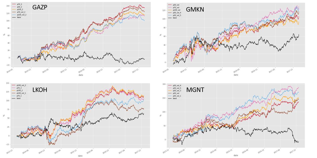
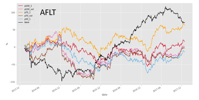
Daily time-series plot of these statistics (black line - SBER price, five colored lines - cumulative co-directionality statistics for top 5 features with the biggest correaltion):
R = pd.DataFrame()
for col in cols.index[:5]:
    R[col] = Z.apply(lambda x: x['tomorrow_change'] if x[col] > 0 else (-1 * x['tomorrow_change']), axis=1)
R['base'] = Z['tomorrow_change']
R.cumsum().plot(style=['#CE1126', '#E26EB2', '#FFA100', '#8D3C1E', '#63B1E5', '#000000'])
plt.ylabel('%')

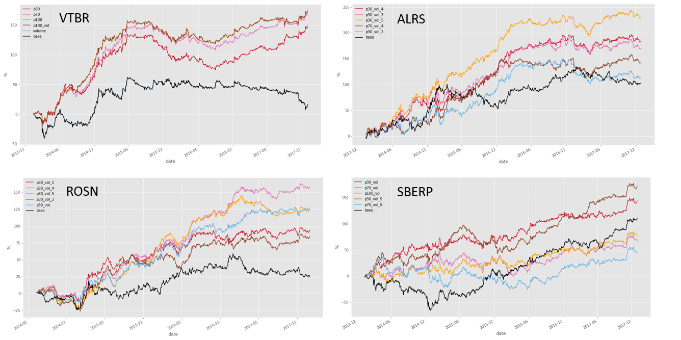
Same plots for other instruments:
Resume
- Using the example of SBER, we calculated the basic statistics, distribution and dynamics of netflow (p30, p70, p100) of large traders in the 2014-2017 period.
- There is strong correlation between net volume and today_change (~ 0.75) and weak correlation with tomorrow_change, but positive and stable (~ 0.1)
- The statistics of one of the indicators of netflow (p70_vol_3) with tomorrow_change (correlation ~ 0.11) is calculated:
Contacts
Website - https://moex.com/en/analyticalproducts?netflow2
Email - support.dataproducts@moex.com